Scrapy, Matplotlib, and MySQL: Real estate data analysis

In this article, we will extract real estate listings from one of the biggest real estate sites and then analyze the data.

Similar to our previous web data analysis blog post, I will show you a simple way to extract web data with python and then perform a descriptive analysis on the dataset.

Tech stack and methodology

We are going to use python as a programming language.

Tools and libraries:

• Scrapy for web scraping
• MySQL to store data
• Pandas to query and structure data in code
• Matplotlib to visualize data

Although this could be a really complex project as it involves web scraping and data analysis as well, we are going to make it simple by using this process:

1. Define data requirements
2. Implement data extraction
3. Perform data analysis (query database + visualization)

Let’s start!

Data requirements

For every web scraping project the first question we need to answer is this - What data do we exactly need? When it comes to real estate listings, there are so many data points we could scrape that we would have to really narrow them down based on our needs. For now, I’m going to choose these fields:

• listing type
• price
• house size
• city
• year built

These data fields will give us the freedom to look at the listings from different perspectives.

Data extraction

Now that we know what data to extract from the website we can start working on our spider.

Installing Scrapy

We are using Scrapy, the web scraping framework for this project. It is recommended to install Scrapy in a virtual environment so it doesn’t conflict with other system packages.

Create a new folder and install virtualenv:

mkdir real_estate cd real_estate pip install virtualenv virtualenv env source env/bin/activate 

Install Scrapy:

pip install scrapy 

If you’re having trouble with installing scrapy check out the installation guide.

Create a new Scrapy project:

scrapy startproject real_estate 

Inspection

Now that we have scrapy installed, let’s inspect the website we are trying to get data from. For this, you can use your browser’s inspector. Our goal here is to find all the data fields on the page, in the HTML, and write a selector/xpath for them.

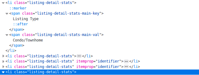
This HTML snippet above contains many list elements. Inside each <li> tag we can find many of the fields we’re looking for, for example, the listing_type field. As different listings have different details defined we cannot select data solely based on HTML tags or CSS selectors. (Some listings have house size defined others don’t) So for example, if we want to extract the listing type from the code above, we can use XPath to choose the one HTML element which has the “Listing Type” in its text then extract its first sibling.

Xpath for listing_type:

"//span[@class='listing-detail-stats-main-key'][contains(text(),'ListingType')]/following-sibling::span"

Then, we can do the same thing for house size, etc…

"//span[@class='listing-detail-stats-main-key'][contains(text(),HouseSize)]/following-sibling::span"

After finding all the selectors, this is our spider code:

def parse(self, response): item_loader = ItemLoader(item=RealEstateItem(), response=response) item_loader.default_input_processor = MapCompose(remove_tags) item_loader.default_output_processor = TakeFirst() item_loader.add_value("url", response.url) item_loader.add_xpath("listing_type", "") item_loader.add_css("price", "") item_loader.add_css("price", "") item_loader.add_xpath("house_size", "") item_loader.add_css("city", "") item_loader.add_xpath("year_built","") return item_loader.load_item() 

As you can see, I’m using an ItemLoader. The reason for this is that for some of the fields the extracted data is messy. For example, this is what we get as the raw house size value:

2,100 sq.ft. 

This value is not usable in its current form because we need a number as the house size. Not a string. So we need to remove the unit and the comma. In scrapy, we can use input processors for this. This is the house_size field with a cleaning input processor:

house_size = Field( input_processor=MapCompose(remove_tags, strip, lambda value: float(value.replace(" sqft", "").replace(",", ""))) ) 

What this processor does, in order:

1. Removes HTML tags
2. Removes unnecessary whitespaces
3. Removes “sqft”
4. Removes comma

The output becomes a numeric value that can be easily inserted into any database:

[insert code]2100 

After writing the cleaning functions for each field, this is what our item class looks like:

class RealEstateItem(Item): listing_type = Field( input_processor=MapCompose(remove_tags, strip) ) price = Field( input_processor=MapCompose(remove_tags, lambda value: int(value.replace(",", ""))) ) house_size = Field( input_processor=MapCompose(remove_tags, strip, lambda value: float(value.replace(" sqft", "").replace(",", ""))) ) year_built = Field( input_processor=MapCompose(remove_tags, strip, lambda value: int(value)) ) city = Field() url = Field() 

Database pipeline

At this point we have the data extraction part handled. To prepare the data for analysis we need to store it in a database. For this, we create a custom scrapy pipeline. If you are not sure how a database pipeline works in scrapy, have a look at this article.

class DatabasePipeline(object): def __init__(self, db, user, passwd, host): self.db = db self.user = user self.passwd = passwd self.host = host @classmethod def from_crawler(cls, crawler): db_settings = crawler.settings.getdict("DB_SETTINGS") if not db_settings: raise NotConfigured db = db_settings['db'] user = db_settings['user'] passwd = db_settings['passwd'] host = db_settings['host'] return cls(db, user, passwd, host) def open_spider(self, spider): self.conn = MySQLdb.connect(db=self.db, user=self.user, passwd=self.passwd, host=self.host, charset='utf8', use_unicode=True) self.cursor = self.conn.cursor() def process_item(self, item, spider): sql = "INSERT INTO Listing (url, price, listing_type, house_size, year_built, city) VALUES (%s, %s, %s, %s, %s, %s)" self.cursor.execute(sql, ( item.get("url"), item.get("price"), item.get("listing_type"), item.get("house_size"), item.get("year_built"), item.get("city") ) ) self.conn.commit() return item def close_spider(self, spider): self.conn.close() 

Now we can run our spider:

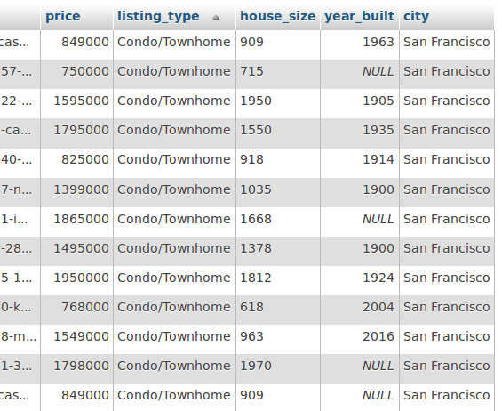
[insert code]scrapy crawl real_estate 

If we’ve done everything correctly we should see the extracted records in the database, nicely formatted.

Data analysis

Now we are going to visualize the data. Hoping to get a better understanding of it. The process we are going to follow to draw charts:

1. Query the database to get the required data
2. Put it into a pandas dataframe
3. Clean, manipulate data if necessary
4. Use panda's plot() function to draw charts

A few important things to point out before drawing far-reaching conclusions while analyzing the dataset:

• We have only ~3000 records (I did not scrape the whole website only part of it)
• I removed the land listings (without a building)
• I scraped listings from only 9 cities in the US

Descriptive reports

Starting off, let’s “get to know” our database a little bit. We will query the whole database into a dataframe and create a new dictionary to get min, max, mean and median values for all numeric data fields. Then create a new dataframe from the dict to be able to display it as a table.

[insert code]query = ("SELECT price, house_size, year_built FROM Listing") df = pd.read_sql(query, self.conn) d = {'Mean': df.mean(), 'Min': df.min(), 'Max': df.max(), 'Median': df.median()} return pd.DataFrame.from_dict(d, dtype='int32')[["Min", "Max", "Mean", "Median"]].transpose()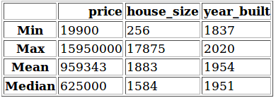 

This table shows us some information:

• The oldest house was built in 1837
• The cheapest house is $19 900, the most expensive is $15 950 000
• The smallest house is 256 sq ft, the largest one is 17 875 sq ft
• The average house was built in the 1950s
• The average house size is 1883 sq ft (174 m2)

Ratio of house types

Overall, we have three types of listings: Condo/Townhome, Multi-family, and Single-family. Let’s see which are the more popular among the listings.

query = ("SELECT listing_type, COUNT(*) AS 'count' FROM Listing GROUP BY listing_type") df = pd.read_sql(query, self.conn, index_col="listing_type") df.plot.pie(y="count", autopct="%1.1f%%", figsize=(7, 7)) plt.show()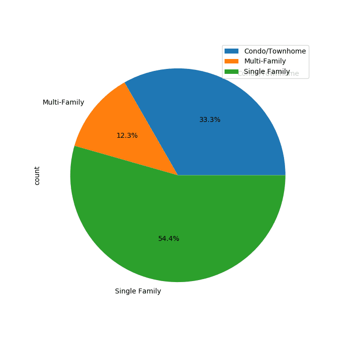 

A little more than half of the listings are Single-family homes. About a third of them are considered Condo/Townhome. And only 12.3% is a Multi-family home.

Correlation between price and year

Next, let’s have a look at the prices. It would be good to see if there’s any correlation between the price and the age of the building.

query = "SELECT price, year_built FROM Listing" df = pd.read_sql(query, self.conn) x = df["year_built"].tolist() y = df["price"].tolist() c = Counter(zip(x, y)) s = [10 * c[(xx, yy)] for xx, yy in zip(x, y)] df.plot(kind="scatter", x="year_built", y="price", s=s, color="blue") yy, locs = plt.yticks() ll = ['%.0f' % a for a in yy] plt.yticks(yy, ll) plt.show()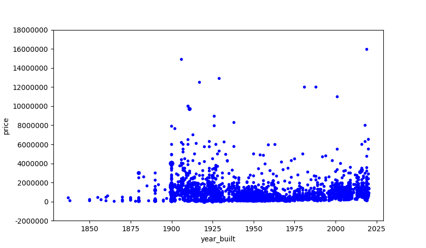 

What we see here is that we have a listing for pretty much every year. But there’s not really a clear conclusion we can draw from this. It looks like there are quite a few houses that were built in the first half of the 20th century and they are more expensive than recently built ones.

Average price per city

In this one, we look at the price tags for each city.

query = "SELECT FLOOR(AVG(price)) AS 'price', city, COUNT(city) AS 'count' FROM Listing GROUP BY city HAVING count > 30" df = pd.read_sql(query, self.conn) df = df.drop(df.index[1]) ax = plt.gca() ax.get_yaxis().get_major_formatter().set_useOffset(False) ax.get_yaxis().get_major_formatter().set_scientific(False) df.plot.barh(x="city", y="price", color="royalblue", ax=ax, grid=True) plt.xlabel("AvgPrice ($)") plt.ylabel("City") plt.show()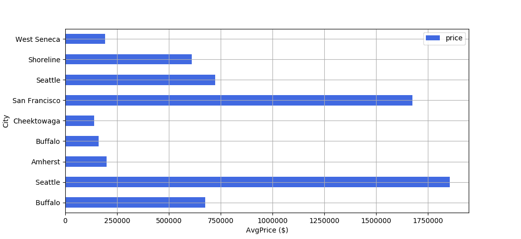 

Among the cities we analyzed, San Francisco and Seattle are the most expensive ones. San Francisco has an average house price of ~$1 650 000. For Seattle, it’s ~$1 850 000. The cheapest cities to buy a house are Cheektowaga and Buffalo, the average price is about $250 000 for both.

Average price per house type

In the next analysis, we examine the average price for different house types. Out of the three house types, which one is the most expensive and the cheapest one?

query = "SELECT FLOOR(AVG(price)) AS 'price', listing_type FROM Listing GROUP BY listing_type" df = pd.read_sql(query, self.conn) ax = plt.gca() df.plot(kind="bar", x="listing_type", y="price", color="royalblue", ax=ax, grid=True, rot=0) plt.xlabel("Type") plt.ylabel("AvgPrice ($)") plt.show()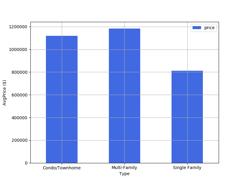 

As we can see, there’s not much of a difference between Condo/Townhome and Multi-Family Type houses.

Both are between $1,000,000 - $ 1,200,000. Single Family homes are considerably cheaper, with an average price of $800,000.

Wrapping up

As I said at the beginning, the data sample I used to create these charts is really small. Thus, the results of this analysis cannot be considered reliable to generalize to the whole real estate market. The goal of this article is just to show you how you can make use of web data and turn it into actual insights.

Want to know how you can use web extracted real-estate data to transform your business? Check out our whitepaper - Fueling real estate’s big data revolution with web scraping

If you have a data-driven product that is fuelled by web data, read more about how Zyte (formerly Scrapinghub) can help you!